

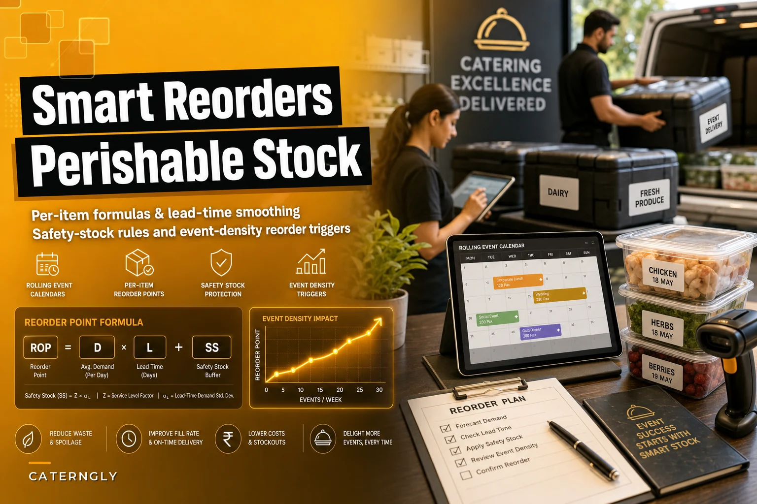

Most caterers track inventory wrong. They count Monday, order Tuesday, then scramble Thursday when overlapping events drive large demand early in the week. This guide keeps a practical operations voice but adds precise notation, canonical inventory formulas (with units), two worked numeric examples (continuous-review ROP plus single-period newsvendor), multi-supplier math, a small Monte-Carlo recipe, and concrete automation assets (data schema, SQL, pseudocode, webhooks).
If you want to jump to implementable assets, I can produce a spreadsheet template (CSV/XLSX) or a runnable Python notebook and the webhook/PO pseudocode for your dev team. Publish the worksheet on a public URL (GitHub/Drive) so your automation can call it.
Notation & assumptions (read this first)
State these symbols and units explicitly in your spreadsheet or code. FEFO allocation and consistent units (portions vs kg) are assumed unless noted otherwise.
-
t — day index (integer). Units
days.
-
L — supplier lead time (days). If variable, L is a random variable with E[L] and Var(L) (days, days^2).
-
S — shelf life / usable life after receipt (days).
-
μ_t — expected demand on calendar day t (units; e.g., portions or kg). Keep units consistent across SKU calculations.
-
σ_t^2 — variance of demand on day t (units^2).
-
DL — demand during the lead-time window; for fixed L
DL = Σ{i=1..L} D{t+i} (units).
-
μD, σD — mean and standard deviation of demand over the period of interest (units).
-
z — standard normal service factor (e.g., 95% service → z ≈ 1.645).
-
Cu — underage cost per unit (lost profit or rush procurement). Currency/unit.
-
Co — overage cost per unit (procurement cost − salvage). Currency/unit.
-
Φ, Φ^{-1}, φ — standard normal CDF, inverse CDF, and PDF.
-
on_hand — current usable inventory (units), excluding items past use-by date.
-
on_order — units already ordered and inbound (expected arrival date(s) required).
-
FEFO assumed
First-Expire-First-Out (allocate from earliest expiry lots).
-
Independence assumptions stated where used; if demand across days is correlated, use scenario methods or Monte-Carlo.
-
Portions ↔ weight
maintain a per-SKU conversion field (e.g., portionsperunit, kgperportion).
Core idea (in one line)
Compute time-phased demand across your exact protection window (lead time + review), compute variability of that demand, pick protection level (z) by a service-level or newsvendor fractile, then enforce perishable caps (don’t order more than you can use before expiry) plus MOQs/lot-size/storage constraints.
End chaos with centralized catering management.
Caterngly helps you plan, confirm, and manage every catering event seamlessly.
- Unified event and order management
- Real-time client updates
- Staff and resource scheduling
No credit card required
When heuristics are used I flag them and show how to tune them from data.
Canonical formulas (with derivations and units)
-
Expected demand during fixed lead time L (units)
E[DL] = Σ{i=1..L} μ_{t+i}. Interpretation: sum the forecasted daily demand that occurs while an order placed today is in transit.
-
Variance of demand during lead time (independent daily forecasts) (units^2)
Var(DL) = Σ{i=1..L} σ{t+i}^2. σD = sqrt(Var(D_L)) (units).
-
Safety stock (fixed L, independent days) (units)
SS = z × σD. ROP = E[DL] + SS.
-
Stationary daily demand (quick checks)
if per-day mean μ and sd σ and fixed L: E[DL] = L × μ, σD = sqrt(L) × σ, SS = z × sqrt(L) × σ.
-
Variable lead time (demand & lead time random)
if daily demand mean μ and sd σ and lead time L has E[L], Var(L) then Var(DL) = E[L] × σ^2 + μ^2 × Var(L). σD = sqrt(Var(DL)); SS = z × σD; ROP = E[L] × μ + SS.
-
Single-period perishable (Newsvendor) — ordering to cover one bounded selling window: Cu = underage cost, Co = overage cost, critical fractile α = Cu / (Cu + Co), z = Φ^{-1}(α), optimal Q* = μD + z × σD (units).
-
Expected spoilage for an order I vs D ~ N(μ,σ^2)
E[spoilage] = (I − μ) Φ((I − μ)/σ) + σ φ((I − μ)/σ) (units).
Perishable caps: hard cap on order arriving at day a: MaxUsefula = Σ{i=1..S} μ_{a+i} + optional buffer. If uncapped SS > MaxUseful, set SS = MaxUseful or change frequency/split deliveries.
Replacing the ambiguous 'Lead Time Weight' with precise, bounded definitions
-
Binary (strict lead-time coverage)
w_e = 1 if DaysUntilEvent ≤ L (event falls inside lead-time window for an order placed today), else 0. Use when you must fully cover an event only if it occurs before the next delivery.
-
Fractional / prepable share (bounded [0,1])
set we = fraction of event demand that must be ordered now; example: delicate greens we = 0, onions we = 1, proteins we = 0.6.
-
Time-phased exact demand
compute exact fraction of event demand that falls into item's usable window after arrival. If arrival a and shelf life S, event on e is useful if e ∈ [a, a+S−1]. This is most precise when modeling arrival dates explicitly.
Pick the definition matching your operations and encode it in your forecasting/ordering engine. Binary and time-phased are statistically grounded; fractional is an operational convenience when you have reuse estimates.
Worked Example A — Continuous‑review ROP with overlapping events (step-by-step)
Assumptions: units = portions. Today = day 0. Lead time L = 2 days (arrive start of day 2). Shelf life S = 5 days. Baseline μbase = 50/day, σbase = 15/day. Event uplifts: day1 +60 (sd 20), day2 +80 (sd 25). Independent day-to-day errors. Desired service level 95% → z = 1.645. We'll compute ROP and check shelf-life cap.
-
Step 1 — daily expected demand inside lead time (days 1..2)
μday1 = 50 + 60 = 110; μday2 = 50 + 80 = 130; E[D_L] = 110 + 130 = 240 portions.
-
Step 2 — variance per day (add independent components)
Varbaseline = 15^2 = 225. Varevent1 = 20^2 = 400 → Varday1 = 625 (σday1 = 25). Varevent2 = 25^2 = 625 → Varday2 = 850 (σday2 ≈ 29.154). Var(DL) = 625 + 850 = 1475 → σ_D ≈ 38.41.
-
Step 3 — safety stock and ROP
SS = z × σD = 1.645 × 38.41 ≈ 63.2 → round SS = 63. ROP = E[DL] + SS = 240 + 63 = 303 portions.
-
Step 4 — shelf-life cap check
MaxUseful (arrive day 2) sum days 2..6. Given day2=130, day3=50, day4..6 baseline 50 each → MaxUseful = 130 + 50 + 150 = 330. Since ROP (303) < MaxUseful (330) no hard cap triggers.
Interpretation: if usable inventory + on_order ≤ 303 portions today, trigger an order to cover the 2-day protection window at 95% service. Round to lot sizes, apply MOQ and storage constraints. Caveats: independence and normal approximations; if event forecasts are skewed use Poisson/NegBin or Monte-Carlo.
Worked Example B — Single‑period perishable (Newsvendor) for Salmon
Scenario: single delivery covers a single selling window then spoils. Units = portions. Demand D ~ Normal(μD = 120, σD = 30). Procurement cost = $12/portion. Salvage = $0. Emergency underage cost Cu = $18. Overaged Co = $12. Critical fractile α = 18/(18+12) = 0.6 → z ≈ 0.253.
-
Step 1 — newsvendor order quantity
Q = μD + z × σD = 120 + 0.253 × 30 = 127.59 → round Q = 128 portions.
-
Step 2 — expected spoilage if I = 128
zspoil = (128 − 120)/30 ≈ 0.2667. Φ(zspoil) ≈ 0.6055; φ(z_spoil) ≈ 0.3849. E[spoilage] = (8)×0.6055 + 30×0.3849 ≈ 16.39 portions. Expected spoilage cost ≈ 16.39 × $12 = $196.7. Stockout probability ≈ 1 − 0.6055 = 0.3945.
Interpretation: Q* minimizes expected combined cost of spoilage and stockouts given Cu/Co. Use exact distributions or Monte-Carlo if normality is suspect; include true salvage/emergency labor/freight costs.
Multi‑supplier example: lead‑time variance & vendor‑adjusted safety stock
Situation: SKU can be supplied by A (lead 1 day, prob 0.7) or B (lead 3 days, prob 0.3). Calculate E[L], Var(L) and Var(DL) using Var(DL) = E[L]σ^2 + μ^2 Var(L).
-
E[L] = 0.7×1 + 0.3×3 = 1.6 days; E[L^2] = 0.7×1 + 0.3×9 = 3.4; Var(L) = 3.4 − 1.6^2 = 0.84 days^2.
-
If μ = 40/day, σ = 10/day
Var(DL) = 1.6×100 + 1600×0.84 = 160 + 1344 = 1504 → σD ≈ 38.79. For z=1.645 SS ≈ 63.8 units.
-
Compare to ignoring LT variability
SS_stationary = z × σ × sqrt(E[L]) ≈ 1.645×10×sqrt(1.6) ≈ 20.8 units. Lead-time variability materially increases SS.
Operational responses: contract for predictable LT, hold vendor-adjusted SS, or split deliveries. A heuristic: prioritize vendor-adjusted SS when SSwithvar > 2×SSwithoutvar or Var(L) contributes >50% of Var(D_L) — test in a pilot before adopting.
Split orders vs consolidated orders — decision logic & numeric split example
Objective: minimize expected spoilage + expected emergency order cost. Key levers: shelf life S, demand time profile, supplier delivery days / MOQs, holding cost h, emergency premium Pe.
-
Rule matrix starters
if S is short relative to gap between events → prefer split deliveries; if MOQ forces large orders and expiry risk is high → negotiate smaller lots or plan transfers; if emergency premium Pe is large → bias toward higher SS or more frequent orders.
-
Worked salmon split (concrete)
Saturday+Sunday demand 180 portions (arrives Thu). Tuesday demand 161 (arrives Mon). S = 4 days. If you order all 341 for Thu, Tue share will be too old. Split Thu: 180, Mon: 161. If supplier MOQ = 200, consider cost of spoiling the 20 extra vs rush penalty — compute expected spoilage using the formula to decide.
Practical automation recipes (data schema, SQL, pseudocode, webhooks)
Minimum data schema (CSV/DB fields) to implement formulas and automation. Keep event forecasts as a table with event-level expectedportions and sd so you can aggregate to daily μt and σ_t.
| field | type / notes |
|---|---|
| sku_id | string |
| sku_name | string |
| unit_type | portions | kg |
| portionsperunit | conversion for consistent units |
| shelflifedays | S |
| supplier_id | string |
| supplierleadtimedaysmean | E[L] |
| supplierleadtimedayssd | sd(L) |
| minorderqty / lot_size | MOQs & lot rounding |
| onhand / onorder | current usable / inbound units (with ETA) |
| event_forecasts table | eventid, eventdate, skuid, expectedportions, sdportions, committedbool |
Sample SQL to compute E[DL] and Var(DL] for sku X today (pseudocode): SELECT skuid, SUM(mu) AS EDL, SUM(sigma2) AS VarDL FROM forecast WHERE skuid = 'SKU123' AND date BETWEEN DATEADD(CURDATE(), INTERVAL 1 DAY) AND DATE_ADD(CURDATE(), INTERVAL @L DAY);
Python pseudocode: continuous-review trigger (summary of steps). 1) compute EDL and VarDL; 2) sigmaD = sqrt(VarDL); 3) SS = z * sigmaD; 4) ROP = EDL + SS; 5) enforce shelf-life cap; 6) recommendedorder = max(0, ROP − onhand − onorder); 7) apply lotsize and minorderqty; 8) check storage capacity; 9) output recommendation.
Event-driven webhook flow (simple): 1) Booking/PMS → POST /api/forecast with per-event per-SKU expectedportions. 2) Forecast service updates forecast table and recomputes ROPs. 3) Inventory engine receives /api/inventory/alerts with recommendedorder and action. 4) Supplier system receives PO via webhook/EDI (if auto_order) or ops receives alert for manual approval. Example webhook payload (to supplier) preserved for copy/paste in implementation.
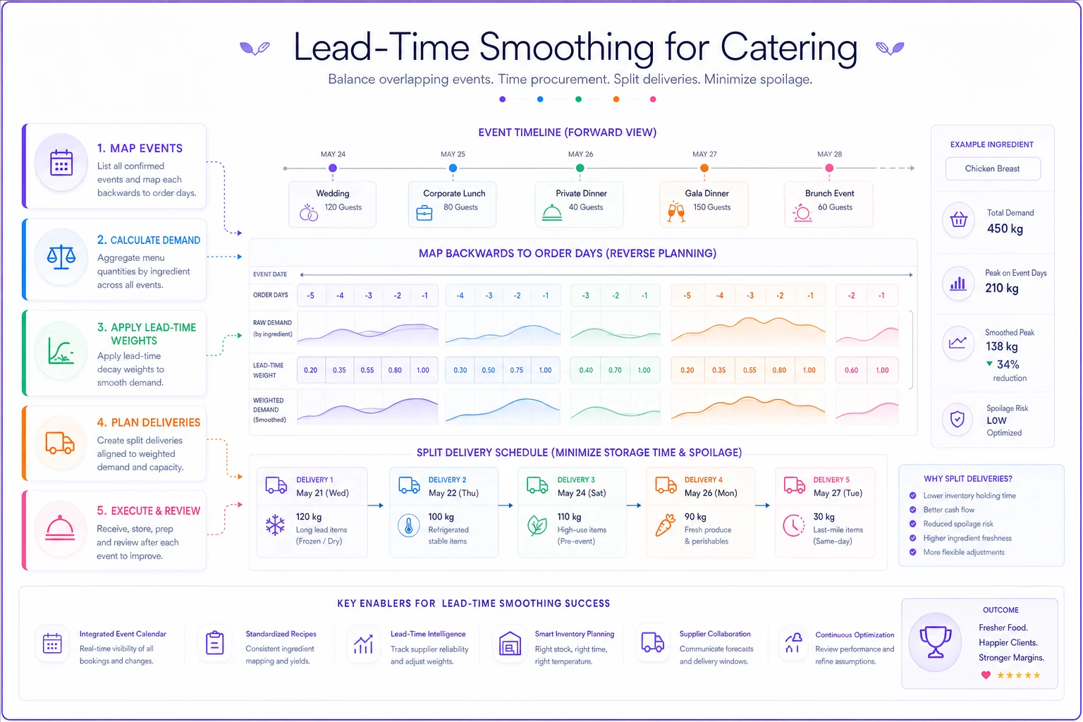
Monte‑Carlo appendix (Python sketch ~30 lines) — simulate overlapping events, compare policies
Purpose: validate ROP and split-order policies under realistic non-normal event patterns. Use numpy/pandas; sample daily demand as Normal or Poisson depending on SKU; simulate Nsim scenarios; for each policy simulate inventory flows (FEFO), spoilage, emergency orders and total cost; compare mean and percentiles.
-
Inputs
Nsim, horizondays, daily μt and σt arrays, lead time L, shelf life S, policy definitions, emergencycostperunit, spoilagecostper_unit, holding cost.
-
Sim
for each sim draw Dt (Normal or Poisson), apply policy ordering logic, simulate arrivals, allocate FEFO, compute spoilage and emergency orders, accumulate totalcost.
-
Output
compare mean total_cost for policies, percentiles, and KPI deltas. Use Poisson/bootstrap for low counts and empirical lead-time distribution where available.
Operational constraints and how they modify order quantities
-
Supplier MOQs and lot sizes → round recommended order to nearest lot; communicate partial fills.
-
Storage capacity by temperature zone → cap daily deliveries to not exceed capacity.
-
Prep labor windows → effective lead time = max(supplier lead, nextprepdate − today).
-
Minimum order frequency / fixed per-order fees → include per-order fixed cost if optimizing consolidation.
-
Adjusted order formula (pseudo)
Qunconstrained = max(0, ROP − onhand − onorder); Qlotted = max(minorderqty, ceil(Qunconstrained / lotsize) * lotsize); Qcapacity = min(Qlotted, storagecapacityremaining); if Qcapacity < Q_unconstrained flag for split or transfer.
FEFO / lot tracking and allocation algorithm
Rules: Receive and stamp lots with arrivaldate and useby = arrivaldate + shelflifedays. Allocate from earliest useby. When computing onhand for decisions, count only units with remaining shelf life ≥ minimumrequireddaysforupcomingevent. Safety stock must account for usableonhand in soon-expiring lots.
-
For event e on day d requiring Qe
while Qe > 0 select lot with smallest useby ≥ d and allocate min(lot.remainingunits, Qe). Update lot.remainingunits and Q_e.
-
If Q_e > 0 after exhausting usable lots → shortage → trigger emergency order logic.
-
When computing usableonhand for SS reduction, include only lots with useby ≥ eventdate.
KPI definitions and monitoring dashboard guidance
-
spoilagerate = wastedunits / units_received (daily/weekly by SKU)
-
emergencyorderrate = numberofemergencyorders / totalorders
-
forecasterrorby_event (MAPE) = mean(|actual − forecast| / actual) across events
-
stockoutspersku = count(stockout_days) per period
-
carryingcostpersku = avginventoryunits × costperunitper_day
-
fillratebyevent = 1 − (unfilledportions / requested_portions)
-
ontimedelivery_rate (supplier-level)
Suggested two-week pilot (top-5 SKUs): collect shelf life and historical event demand, run ROP & newsvendor calculations and Monte-Carlo comparisons, start with alert-only for week 1 then enable auto-orders week 2 if ops sign-off and low false-positive rate.
Assumptions & limitations (when formulas break)
Common failure modes: independence assumptions, poor normal approximations for low counts or skewed events, sparse data for new SKUs, lead-time nonstationarity, and poor data quality for bookings vs committed orders. When in doubt, simulate (Monte-Carlo) rather than rely solely on closed forms.
-
Independence
Var(DL) = Σσt^2 assumes day-to-day independence. Add covariance terms or scenario sampling if correlated.
-
Distribution tails
normal approximation may be poor for low counts; prefer Poisson/NegBin/bootstrap.
-
Sparse data
estimate σ_t using similar SKUs or conservative CV until you collect data.
-
Lead time nonstationarity
use rolling windows for E[L] and Var(L) when supplier behavior changes.
Practical deployment checklist (short)
-
Instrument
ensure event system emits per-event per-SKU expected usage and confidence.
-
Baseline
compute historical μt and σt per day-of-week and event-type.
-
Implement
ROP/SS calculator as a service or spreadsheet using formulas above.
-
Integrate
booking/PMS → Forecast service → Inventory engine → Supplier PO API (webhook).
-
Enforce FEFO and date-marking on receipt (FDA Food Code reference included above).
-
Pilot
run top-5 SKUs for two weeks with flags only, then enable auto-orders if safe.
-
Iterate
tune z or Cu/Co and split rules using measured spoilage & emergency rates.
Final operational advice
Start with 5 SKUs (produce, fresh fish, frozen protein, dairy, high-value garnish). Instrument event forecasts (committed vs tentative), enforce FEFO and date-marking, use canonical formulas; where data are sparse run Monte-Carlo or bootstrap. When supplier variability drives SS up materially, evaluate commercial or operational alternatives (more reliable vendor, smaller lots, split deliveries).
Measure outcomes (spoilagerate, emergencyorder_rate) and tune z / Cu/Co from real cost data rather than gut feel.
If you'd like, I can: (A) produce the spreadsheet template (CSV/XLSX) implementing these formulas and the worked examples ready to publish; (B) generate the runnable Python Monte‑Carlo notebook (Jupyter) that implements the simulation pseudocode and prints policy comparisons; or (C) produce packaged pseudocode and webhook/PO payload examples for your dev team. Which deliverable would you like first?
Ready to elevate your catering business?
Join 500+ caterers trusting Caterngly to save time, reduce errors, and deliver flawless events.